RDDL Language Description

Introduction

The Relational Dynamic Influence Diagram Language (RDDL) is a uniform language where states, actions, and observations (whether discrete or continuous) are parameterized variables and the evolution of a fully or partially observed (stochastic) process is specified via (stochastic) functions over next state variables conditioned on current state and action variables (n.b., concurrency is allowed). Parameterized variables are simply templates for ground variables that can be obtained when given a particular problem instance defining possible domain objects.

Semantically, RDDL is simply a dynamic Bayes net (DBN) (with potentially many intermediate layers) extended with a simple influence diagram (ID) utility node representing immediate reward. An objective function specifies how these immediate rewards should be optimized over time for optimal control. For a ground instance, RDDL is just a factored MDP (or POMDP, if partially observed).

File Structure and Syntax

Domain Block

The domain block defines the domain of a problem that will be used to perform simulations accordingly. The objects, states and actions to be simulated, and the rules that the simulations should follow, are all defined in this block. The block should be written in a .rddl file as the following:

domain <domain_name> {
    requirements { <code> };
    types { <code> };
    pvariables { <code> };
    cpfs { <code> };
    reward = <code>;
    state-invariants { <code> }; // optional
    action-preconditions { <code> }; // optional
    termination { <code> }; // optional
}

Note

There should not be a semicolon at the end of the domain block.

Requirements

The requirements section of the domain block states the characteristics of the domain. Specifically, the requirements section tells the parser what kind of parameterized variables will be defined, what types of values (integer, real numbers or user defined values) the variables will be assigned to, and how the actions and reward will be determined.

The requirements section will be included in the .rddl file with the following format:

requirements { <requirement1>, <requirement2>, ... };

There are currently nine requirements that can be implemented in RDDL, as shown in the following table:

Possible Requirements
requirement	representation
concurrent	This domain permits multiple non-default actions
constrained-state	This domain uses state constraints
continuous	This domain uses real-valued parameterized variables
cpf-deterministic	This domain uses deterministic conditional functions for transitions (it is important to note that RDDL can also be used to model deterministic domains)
integer-valued	This domain uses integer variables
intermediate-nodes	This domain uses intermediate parameterized variable nodes
multivalued	This domain uses enumerated parameterized variables
partially-observed	This domain uses observation parameterized variables so it is treated as a POMDP (not an MDP as is otherwise the case)
reward-deterministic	This domain does not use a stochastic reward

Types

The types section defines the objects and user defined values, if any, that will be used in the domain, according to the following format:

types {
    <object1> : object;
    <object2> : object;
    ...

    <enumerable> : {@<value1>, @<value2>, ... };
};

An object is a user-defined parameter that will be used to parameterize variables. They are often things or people that will be simulated to move or act in this domain.

For example, consider a simulation where elevators are to travel between different floors and open doors to allow people to get on and off the elevators to ultimately minimize the waiting time (see elevators.rddl example). person and elevator can be declared as objects in the domain as follows:

types {
    person : object;
    elevator : object;
};

The @ quantifier specifies that the given value should be treated as an object rather than a pvariable. This symbol is generally optional for objects in expressions, however:

Warning

If the @ symbol is not prepended to an object, and there is a variable defined in the domain with the same name as the object that does not have parameters, then it is ambiguous whether the object or the variable are being referred to inside an expression. The compiler will raise an exception in this case.

Parameterized Variables (pVariables)

This section is included to declare all variables used in the domain. These variables include constant values, states and action variables, as well as potentially intermediate and observed variables. Ultimately, these variables will serve as condition-determining parameters in transitions of states. The variables declared in this section can be either parameterized by one or more objects, or non-parameterized, and they are declared according to the following format:

pvariables {

    // parameterized variables
    <pvariable1>(<obj1>, [<obj2>, ...]) : { <type_fluent>, <type_value>, default = <value> };
    <pvariable2>(<obj1>, [<obj2>, ...]) : { <type_fluent>, <type_value>, default = <value> };
    ...

    // non-parameterized variables
    <variable1> : { <type_fluent>, <type_value>, default = <value> };
    <variable2> : { <type_fluent>, <type_value>, default = <value> };
    ...
};

The <type_fluent> argument specifies the function of the variable declared. This argument can take one of the following five values:

non-fluent: variable that never changes during a simulation. Non-fluents will be initialized in the non-fluents block before simulation starts
state-fluent: or state variable, variable that represents the state of a simulation, often used to describe the state or relative state of objects (e.g., locations, occupancy, etc.).
interm-fluent: or intermediate variable, variable that is used as an intermediate conditional probability calculation. Intermediate fluents must have a level of stratification, and are strictly stratified so that an intermediate variable can only condition on intermediate variables of a strictly lower level or state variable.
observ-fluent: or observation variable, variable used as a conditional observation probability in partially observable Markov decision process (POMDP).
action-fluent: or action variable, variable that represents the action of a simulation, often used to describe if a transition between two different states is happening.

The <type_value> argument specifies the values the declared variable can take on. This argument can be one of the following four options:

bool: boolean valued variable (i.e., true, false). Note that these variables are evaluated to 1 or 0 when used in arithmetic expressions
int: integer valued variable (i.e., 1, 2, 3, 10, 100 …)
real: real valued variable (i.e., 0.1, 0.25, 1.414, 2.718, 3.142 …)
<enumerable>: an enumerated value defined by the user in the types section
<object>: an object type defined in the types section whose objects are specified in the instance (this is a new feature of pyRDDLGym)

The last argument sets a default value to the declared variable. If the variable is a non-fluent or state-fluent and is not specified to have a certain value in the non-fluent or instance block (which will be mentioned in later sections), the variable will take its default value. If the variable is an action-fluent, then when the action is not performed this variable will take on its default value; an action-fluent taking an non-default value would imply the action is performed in most cases. Default values are not specified for interm-fluent and observ-fluent.

Note

In case of a interm-fluent, the old RDDL specification required that the last argument be level = <int> instead, where the integer represents the level of stratification. However, the new RDDL specification no longer requires levels to be specified in the domain, since they are computed automatically at compile time.

Conditional Probability Functions (CPFs)

The cpfs section is the key to describe how the simulation will change the states at each time step: this section contains all state transition functions. The functions describe how each state-fluent at the next time step will vary based on the fluents of the current time step. If this is a stochastic domain, then the cpfs block represents the state-fluents at the next time step with some probability distribution function.

Each state-fluent requires a conditional probability function to represent the value of this state-fluent at the next time step. The state-fluent at the next time step is represented by adding an apostrophe at the end of the state-fluent (i.e., <name_state-fluent>'). If the state-fluent is parameterized by objects, the objects are referenced by a ? followed with user assigned names for the query objects.

For example, if a pvariable elevator-at-floor(elevator, floor) is defined, then elevator-at-floor(?e, ?f) represents the value of this variable parameterized by elevator ?e and floor ?f.

cpfs {
    <cpf1>(<param1>, <param2>, ...) = <expression1>;
    <cpf2>(<param1>, <param2>, ...) = <expression2>;
    ...
};

The function can be constructed using various conditional expressions, logical and arithmetic operators, as well as probability distribution expressions. For example, the following code comes from the elevator control example:

person-waiting-up'(?f) =
    if (person-waiting-up(?f) ^
        ~exists_{?e: elevator} [elevator-at-floor(?e, ?f) ^ elevator-dir-up(?e) ^ ~elevator-closed(?e)])
    then true
        else Bernoulli(ARRIVE-PARAM(?f));

where ?f is a floor object and ?e is an elevator object. This function assigns a value true to the next-time-step person-waiting-up state-fluent if there is already a person waiting and no elevator has arrived to load the person; otherwise there is a Bernoulli probability distribution with ARRIVE-PARAM(?f) chance of a person arriving at the floor and setting the next-time-step person-waiting up state-fluent to be true. Evidently, this models the randomness of people arriving and waiting for an elevator.

Warning

Cyclic dependencies between two or more CPFs, or a CPF expression that refers to itself, is strictly prohibited and will raise an exception.

The usage of all conditional expressions, logical and arithmetic operators, and probability distribution expressions will be described in a later section.

Reward

To properly know which action should be performed, an objective function is needed. This objective function is represented in the domain block as the reward. The reward function should be designed such that the actions are taken to maximize the reward. This is done by assigning a value to reward using state-fluents, interm-fluents, or action-fluents with the following format:

reward = <expression>;

where all conditions must remain true with respect to all actions taken during the simulation.

Action-Preconditions and State-Invariants

The action-preconditions block is used for specifying constraints that restrict single or joint action usage in a particular state and is only checked when an action is executed:

action-preconditions {
    <condition1>;
    <condition2>;
    ...
};

The state-invariants block is used for constraints that do not include any action-fluents and thus represent state property assertions that should never be violated. These constraints are checked in the initial state and every time a next state is reached. The simulator should exit if a state-invariant is violated and hence the author should specify state-invariants as a way to verify expected domain properties.

state-invariants {
    <condition1>;
    <condition2>;
    ...
};

Termination

An Addition made to the RDDL language during the development of this infrastructure is the termination block. This block is intended to specify terminal states in the MDP, which when reached the simulation will end. A terminal state is a valid state of the MDP (to emphasize the difference from state-invariants). An example of terminal state can be any state within the goal set for which the simulation should not continue, or a state where there are no possible actions and the simulation should end. E.g., hitting a wall when it is not allowed. When a terminal state is reached the state is returned from the environment and the done flag is returned as True. The reward is handled independently by the reward function, thus if there is a specific reward for the terminal state, it should specified in the reward formula. The termination block has the following syntax:

termination {
    <terminal_condition1>;
    <terminal_condition2>;
    ...
};

where <terminal_condition#> are boolean formulas. The termination decision is a disjunction of all the conditions in the block (termination if at least one is True).

Valid Dependencies

Fluent variables in RDDL have a strict dependency structure, as outlined in the schematic below:

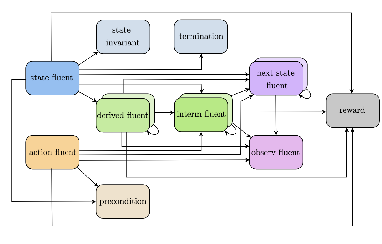
Dependencies between fluents in RDDL documents

In summary:

a non-fluent can be used in any expression
state invariants and termination block are checked in each state, so they are expressed using unprimed state variables
action preconditions are checked for each state-action pair, so they are also expressed using unprimed state variables
derived-fluent is deprecated and should be replaced by interm-fluent
primed state-fluent and interm-fluent can depend on other primed state-fluent and interm-fluent, unless allow_synchronous_state = False
cyclic dependencies (e.g. a fluent expression depends on the value of that fluent) are not allowed.

Non-fluents Block

The non-fluents block defines all objects need and all non-fluent variable values in a problem domain which is specified in the same block. The non-fluents block should have the following syntax:

non-fluents <non-fluents_name> {
    domain = <domain_name>;
    objects {
        <object_name1> : {<obj1>, <obj2>, ... };
        <object_name2> : {<obj1>, <obj2>, ... };
        ...
    };

    non-fluents {
        <non-fluent1> = <value1>;
        <non-fluent2> = <value2>;
        ...
    };
}

Note

There should not be a semicolon at the end of the non-fluents block.

The objects section define all objects needed; these are grouped by types and listed in curly bracket. The non-fluents section lists all non-fluent variables that do not take their default values and assigns a value to them. If the non-fluent variable is parameterized by objects, simply state the parameters in parentheses after the non-fluent, e.g.:

<non-fluent>(<obj1>, <obj2>, ...) = <value>;

non-fluent variables in the domain that are not listed in this section will take their default value stated in the domain block. For simplicity, assigning true to a bool type variable can be achieved by stating the name of the variable; similarly, assigning false to a bool type variable can be achieved by stating the name of the variable with an apostrophe after it, i.e.:

bool_variable1; // same as bool_variable1 = true;
bool_variable2'; // same as bool_variable2 = false;

Instance Block

The instance block defines a specific problem instance to be simulated, by stating the initial states, number of actions that can occur at a single time step (concurrently), as well as the horizon and the discount factor for MDP. It is also specified in this block which domain and non-fluents block this instance is referring to. The instance block should have the following syntax:

instance <instance_name> {
    domain = <domain_name>;
    non-fluents = <non-fluents_name>;
    init-state {
        <state-fluent1> = <value1>;
        <state-fluent2> = <value2>;
        ...
    };
    max-nondef-actions = <int>;
    horizon = <int>;
    discount = <real>;
}

Note

There should not be a semicolon at the end of the instance block.

Any state-fluents that do not take their default value initially should be assigned a value in the init-state section. Similarly as in the non-fluent block, bool type variables can simply be assigned true by calling its name, and assigned false by adding an apostrophe. State-fluent variables in the domain that are not listed in this section will take their default value stated in the domain block.

The max-nondef-actions represents the maximum number of action-fluent there can be at a single time step that are not at their default values, or the maximum number of concurrent actions. Setting this parameter to pos-inf will set the number of concurrent actions equal to the total number of action-fluents.

The horizon and discount factor are parameters for MDP to work on this instance. horizon is the total number of time steps that the instance will be simulated for (e.g., if horizon = 10, the instance will be simulated from time = 0 to time = 9).

The discount represents how much more/less future rewards should be worth compared to the current reward. For example, if discount = 0.9, then 1 point of reward in two time steps after would have the same value as 1 * 0.9 * 0.9 = 0.81 point of reward currently.

Note

A discount factor of less than 1 means earlier rewards are preferred, a discount factor of greater than 1 means later rewards are preferred, and a discount factor of 1 means the reward should have no difference with respect to time.

Functions and Expressions

As of the time of this writing, RDDL syntax supports the following mathematical operations:

Basic Math Functions
RDDL syntax	description
`div[x, y]`	divides `y` by `x` for integer arguments
`mod[x, y]`, `fmod[x, y]`	returns `x % y` for integer and float arguments, respectively
`min[x, y]`, `max[x, y]`	the minimum and maximum, respectively, of `x` and `y`
`abs[x]`	the absolute value of `x`
`sgn[x]`	returns the sign of `x`, e.g. `1 if x > 0; -1 if x < 0; 0 if x == 0`
`round[x]`	rounds `x` to the nearest integer
`floor[x]`	the greatest integer less than `x`
`ceil[x]`	the smallest integer greater than `x`

the following exponential, logarithmic and transcendental functions:

Exponential, Logarithmic and Transcendental Functions
RDDL syntax	description
`log[x, b]`	the logarithm of `x` with base `b`
`ln[x]`	the natural logarithm of `x`
`exp[x]`	the value `e ^ x` where `e` is Euler’s constant
`pow[b, x]`	the value of `b ^ x`
`sqrt[x]`	the square root of `x`
`hypot[x, y]`	the value of `sqrt[pow[x, 2] + pow[y, 2]]`
`gamma[x]`, `lngamma[x]`	the gamma function and its natural log, respectively, evaluated at `x`

and the following trigonometric functions:

Trigonometric Functions
RDDL syntax	description
`cos[theta]`, `sin[theta]`, `tan[theta]`	the cosine, sine and tangent, respectively, of `theta`
`acos[theta]`, `asin[theta]`, `atan[theta]`	the arc cosine, sine and tangent, respectively, of `theta`
`cosh[theta]`, `sinh[theta]`, `tanh[theta]`	the hyperbolic cosine, sine and tangent, respectively, of `theta`

Conditional Expressions

Conditional expressions are necessary to give conditional dependencies to the state-action graphical model. These expressions are almost always necessary when writing conditional probability functions. Currently, RDDL support two types of conditional expressions: if-else and switch.

Equality and Inequality Comparison Expressions

RDDL supports basic comparison expressions including equality (==), disequality (~=), and inequality comparisons (>, <, >=, <=). Equality (==) and disequality (~=) can be used between any identical range variables, while inequality comparisons (>, <, >=, <=) can be used between any numerically valued variables (real, int, and bool).

Warning

Using any of the comparison operators on objects of different types, or mixed object and primitive (e.g. real, int, bool) data types, will raise an exception; this includes equality and disequality operators.

If-then-else

The if-then-else expressions is similar to any if expressions in other programing languages:

if (<condition>) then <expression1> else <expression2>

If <condition> evaluates to true, <expression1> will be used; otherwise, <expression2> will be used.

Each <expression> can also be an if-then-else expression, as shown in the following. Also note that in RDDL, parentheses ( ) and square brackets [ ] serve the same purpose of grouping and are interchangeable.

if (<conditions1>) then [if (<conditions2>) then <expression2> else <expression1>] else <expression2>;
if (<conditions1>) then <expression1> else if (<conditions2>) then <expression2> else <expression2>;

switch

The switch expression can be used if the argument involved in the desired conditions is an enumerated variable. The syntax of this expressions is

switch (<argument>) {
    case @<value1> : <expression1>,
    case @<value2> : <expression2>,
    ...
    default : <default expression>;  // optional
};

This allows RDDL to examine the value of <argument> first, then use the corresponding expression associated with that value.

Note

Note that the default statement must be included if the cases are not exhaustive.

Warning

Multiple cases with the same case value, multiple default statements, or non-exhaustive cases without a default statement, will raise an exception.

Logical Expressions

RDDL supports the logical expressions AND (^), OR (|), NOT (~), IMPLIES (=>), and EQUIVALENCE (<=>) for boolean (binary) variables.

Additionally, RDDL supports the “for all” and “there exists” expressions. The following expression returns true if for all possible (tuples of) objects, <condition> evaluates to true. If there exists any possible (tuple of) objects that would cause <condition> to be false, the expression will return false:

forall_{?<obj1>: <object1_name>, [?<obj2>: <object2_name>, ...]} [<condition>]

The following expression returns true if there exists any possible (tuple of) objects that would cause <condition> to be true. If for all possible (tuples of) objects, <condition> evaluates to false, the expression will return false:

exists_{?<obj1>: <object1_name>, [?<obj2>: <object2_name>, ...]} [<condition>]

Arithmetic Operators and Aggregations

RDDL supports basic binary arithmetic operations using typical symbols: ADD(+), SUBTRACT(-), MULTIPLY(*), and DIVIDE(/).

Arithmetic operations, or “aggregations”, over a sequence of arguments such as sum and product are also supported:

sum_{?<obj1>: <object1_name>, [?<obj2>: <object2_name>, ...]} [<expression>]
prod_{?<obj1>: <object1_name>, [?<obj2>: <object2_name>, ...]} [<expression>]

Note

Unlike the old RDDL specification, it is now possible to aggregate over enumerated (domain object) types in addition to instance-defined objects.

RDDL supports the following aggregations over types:

Aggregations
RDDL syntax	description
`sum_{...} [<expression>]`	the sum of `<expression>`
`prod_{...} [<expression>]`	the product of `<expression>`
`avg_{...} [<expression>]`	the arithmetic average of `<expression>`
`minimum_{...} [<expression>]`	the minimum of `<expression>`
`maximum_{...} [<expression>]`	the maximum of `<expression>`

The new language extension now also supports argmin and argmin with the following syntax:

argmin_{?<obj>: <object_name>} [<expression>]
argmax_{?<obj>: <object_name>} [<expression>]

The first (second) expression returns the index of the object <obj> that minimizes (maximizes) <expression> over all objects in <object_name>.

Note

Unlike aggregations, argmax and argmin iterate over a single parameter only.

Warning

It is required to put a pair of parentheses (...) or [...] around each aggregation, to make sure the correct arithmetic order of operations is been parsed by RDDL. Failure to do this could result in the parser silently compiling expressions that differ from their RDDL specification.

Probability Distributions

CPFs assign value to next state variables using probability distributions. These probability distributions are expressed using keywords with parameters, where all parameters can be expressions.

Discrete Distributions

RDDL currently supports the following discrete (int, bool or enumerated values) probability distributions:

Discrete Probability Distributions
RDDL syntax	description	reparameterizable
`KronDelta(v)`	Places all probability mass on its discrete argument `v`	Yes
`Bernoulli(p)`	Samples a boolean value with given probability of success/true	Yes
`Discrete(var, p)`	Samples an enumerated value with given probability distribution	Yes
`UnnormDiscrete(var, p)`	Same as `Discrete` but where `p` can be non-normalized (e.g. not sum to 1)	Yes
`Poisson(rate)`	Samples an integer value from a Poisson distribution with given rate parameter	No
`Binomial(trials, p)`	Samples an integer value from a Binomial distribution with given number of trials and trial probability of success	No
`NegativeBinomial(successes, p)`	Samples an integer value from a Negative Binomial distribution with required number of successes and trial probability of success	No
`Geometric(p)`	Samples an integer value from a Geometric distribution with given probability of success	Yes

In a Discrete probability distribution, the probability vector assign a probability density to each possible value of the enumerated variable, with the following format:

Discrete(<variable_name>,
    @<value1> : <expression1>,
    @<value2> : <expression2>,
    ...
)

The new RDDL also supports a more compact syntax for Discrete and UnnormDiscrete, which is similar to aggregation:

Discrete_{?<value> : <variable_name>}( <expression>(?<value>) )
UnnormDiscrete_{?<value> : <variable_name>}( <expression>(?<value>) )

where <expression> must be a real-valued expression or pVariable.

Continuous Distributions

RDDL also currently supports the following continuous (real values) probability distributions:

Continuous Probability Distributions
RDDL syntax	description	reparameterizable
`DiracDelta(v)`	Places all probability mass on its continuous argument `v`	Yes
`Normal(mean, variance)`	Samples a continuous value from a Normal distribution with given mean and variance	Yes
`Uniform(lower, upper)`	Samples a real value from a Uniform distribution with given lower and upper bounds	Yes
`Exponential(scale)`	Samples a real value from an Exponential distribution given scale	Yes
`Weibull(shape, scale)`	Samples a real value from a Weibull distribution with given shape and scale parameters	Yes
`Gamma(shape, scale)`	Samples a real value from a Gamma distribution with given shape and scale parameters	`scale` only
`Beta(a, b)`	Samples a real value from a Beta distribution with parameters `a` and `b`	No
`Pareto(shape, scale)`	Samples a real value from a Pareto distribution with given shape and scale parameters	Yes
`Student(df)`	Samples a real value from a Student-t distribution with zero mean, unit scale and degrees of freedom `df`	No
`Gumbel(mean, scale)`	Samples a real value from a Gumbel distribution with given mean and scale parameters	Yes
`Laplace(mean, scale)`	Samples a real value from a Laplace distribution with given mean and scale parameters	Yes
`Cauchy(mean, scale)`	Samples a real value from a Cauchy distribution with given mean and scale parameters	Yes
`Gompertz(shape, scale)`	Samples a real value from a Gompertz distribution with given shape and scale parameters	Yes
`ChiSquare(df)`	Samples a real value from a Chi-Square distribution with degrees of freedom `df`	No
`Kumaraswamy(a, b)`	Samples a real value from a Kumaraswamy distribution with parameters `a` and `b`; this is a reparameterizable analogue of the Beta distribution	Yes

New Language Features

Nested pVariables

Another new language feature of RDDL is the ability to nest pVariable calculations. This offers much greater expressiveness of the RDDL language and allows much more complex reasoning to be carried out using enumerated values. The following is valid syntax

<pvar_1>(..., <pvar_2>(?<value_1>, ?<value_2>, ...),
         <pvar_3>(?<value_1>, ?<value_2>, ...), ..., ?<value1>, ?<value_2>, ...)

provided the types of ?<value_#> match the definition of ?<pvar_#> in the pvariables block.

Nesting can also be performed to arbitrary depth, i.e.

<pvar_1>(<pvar_2>(... <pvar_n>(<?value_1>, ...) ...))

provided the types of the variables are correct.

Finally, it is possible to use a combination of enumerated values, objects and other pVariables as parameters when evaluating a pVariable

<pvar>(<pvar_as_parameter>([?<object1>, ...]), @<enum_value>, ?<object>)

as long as @<enum_value>, ?<object> and <pvar_as_parameter> types match what is required by the outer <pvar>.

Multivariable Distributions

The new RDDL syntax now supports sampling from some well-known multivariable probability distributions. For example, a Dirichlet distribution with parameter vector “alpha” can be parameterized by a pVariable alpha that takes at least one enumerated value. The syntax to sample from this distribution and assign it to a CPF is

<cpf>(?<value>) = Dirichlet[?<value>]( alpha(_) );

where cpf is the name of a CPF (e.g., state-fluent, interm-fluent), _ indicates the argument of alpha that describes where the parameter vector of the Dirichlet distribution is described, and [?<value>] indicates which parameter of <cpf> is to receive the sample from this distribution.

Warning

Unlike the single-variable distributions, samples from multivariable distributions must be assigned to CPFs directly (e.g. cannot be nested inside other expressions). Furthermore, their parameters cannot be compound expressions either, but can refer to any valid CPF.

It is also possible to include an arbitrary number of other parameters from the <cpf> in “alpha”, e.g. the following could be valid syntax:

<cpf>(?<value1>, ?<value2>) = Dirichlet[?<value1>]( alpha(?<value2>, _) );
<cpf>(?<value1>, ?<value2>) = Dirichlet[?<value1>]( alpha(_, ?<value2>) );

provided the types of the required and given arguments in alpha match. These examples could be seen as “batched” sampling, where the parameter ?<value2> not corresponding to the sampled dimension specifies a single sample in the “batch”.

In a similar way, new RDDL also provides a syntax for the Multinomial distribution with given trials trials and probabilities p

<cpf>(?<value>) = Multinomial[?<value>]( trials, p(_) );

the multivariate normal with mean mean and covariance cov

<cpf>(?<value>) = MultivariateNormal[?<value>]( mean(_), cov(_, _) );

and the multivariate Student-t with mean mean, Sigma matrix sigma and degrees of freedom df

<cpf>(?<value>) = MultivariateStudent[?<value>]( mean(_), sigma(_, _), df );

Matrix Operations on pVariables

The new RDDL language allows for matrix linear algebra to be performed over pVariables, as if they were matrices. For example, the determinant of the matrix described by an expression <expression> parameterized by (at least) two values can be written as

det_{?<value1> : <variable_name1>, ?<value2> : <variable_name2>} <expression>( ?<value1>, ?<value2> )

which can be viewed roughly as an aggregation over two variables, corresponding to row and column. As with vectorized sampling, it is also possible to incorporate variables from the outer scope to serve as “batch” dimensions, i.e.

det_{?<value1> : <variable_name1>, ?<value2> : <variable_name2>} <expression>( ?<value1>, ?<value2>, ?<value3>, ... )

The syntax for computing the matrix inverse, pseudo-inverse and Cholesky factor of <expression> is

inverse[ row=?<value1>, col=?<value2> ] <expression>( ?<value1>, ?<value2> )
pinverse[ row=?<value1>, col=?<value2> ] <expression>( ?<value1>, ?<value2> )
cholesky[ row=?<value1>, col=?<value2> ] <expression>( ?<value1>, ?<value2> )

Similar to vectorized sampling, these operations produce a matrix rather than a scalar, so ?<value1> and ?<value2> must be variables defined in the outer scope into which the inverse matrix will be assigned. Also, to break ambiguity between which of ?<value1> and ?<value2> corresponds to the row and column dimensions of <expression>, they must be explicitly assigned to the row and column dimensions as in the code above, i.e. ?<value1> runs over the rows and ?<value2> runs over the columns of the “matrix” produced by <expression>. As with determinant, this calculation can be “batched” if <expression> is appropriately parameterized by other variables from the outer scope.